INTERNSHIP

INTERNSHIP REPORT:
BASIC TASK IN  MS WORD AND MS EXCEL

MS WORD

 Word 2016 is designed to help you create professional-quality documents. Word can also help you organize and write documents more efficiently.

When you create a document in Word, you can choose to start from a blank document or let a template do much of the work for you. From then on, the basic steps in creating and sharing documents are the same. And Word's powerful editing and reviewing tools can help you work with others to make your document great.

Start a document

It’s often easier to create a new document using a template instead of starting with a blank page. Word templates come ready-to-use with pre-set themes and styles. All you need to do is add your content.

Each time you start Word, you can choose a template from the gallery, click a category to see more templates, or search for more templates online.

For a closer look at any template, click it to open a large preview.

If you’d rather not use a template, click Blank document.

Open a document

Every time you start Word, you’ll see a list of your most recently used documents in the left column. If the document you’re looking for isn’t there, click Open Other Documents.

If you’re already in Word, click File > Open and then browse to the file’s location.

When you open a document that was created in earlier versions of Word, you see Compatibility Mode in the title bar of the document window. You can work in compatibility more or you can upgrade the document to use Word 2016. 

Save a document

To save a document for the first time, do the following:

1..On the File tab, click Save As.

2.Browse to the location where you’d like to save your document.

3.Click Save.

To save your document as you continue to work on it, click Save in the Quick Access Toolbar.

To move from page to page in a document, do one of the following:

Read document

Open your document in Read Mode to hide most of the buttons and tools so you can get absorbed in your reading without distractions.

1.Open the document you want to read.

2.Click View > Read Mode. 

3.To move from page to page in a document, do one of the following:

• Click the arrows on the left and right sides of the pages.

• Press page down and page up or the spacebar and backspace on the keyboard. You can also use the arrow keys or the scroll wheel on your mouse.

• If you’re on a touch device, swipe left or right with your finger.

Track changes

When you’re working on a document with other people or editing a document yourself, turn on Track Changes to see every change. Word marks all additions, deletions, moves, and formatting changes.

1. Open the document to e reviewed.

2. Click Review and then on the Track Changes button, select Track Changes.

Print your document

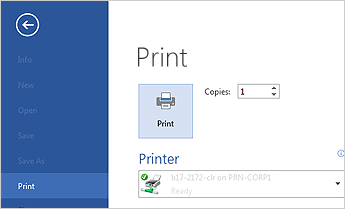
All in one place, you can see how your document will look when printed, set your print options, and print the file.

1. On the File tab, click 
2. Do the following:

• Under Print, in the Copies box, enter the number of copies you want

• Under Printer, make sure the printer you want is selected.

• Under Settings, the default print settings for your printer are selected for you. If you want to change a setting, just click the setting you want to change and then select a new setting.

3.When you’re satisfied with the settings, click Print.

 MS EXCEL

Excel is an incredibly powerful tool for getting meaning out of vast amounts of data. But it also works really well for simple calculations and tracking almost any kind of information. The key for unlocking all that potential is the grid of cells. Cells can contain numbers, text, or formulas. You put data in your cells and group them in rows and columns. That allows you to add up your data, sort and filter it, put it in tables, and build great-looking charts. Let’s go through the basic steps to get you started.

Create a Notebook.

Excel documents are called workbooks. Each workbook has sheets, typically called spreadsheets. You can add as many sheets as you want to a workbook, or you can create new workbooks to keep your data separate.

1. Click File, and then click New.

2. Under New, click the Blank workbook.

Enter Your Data

1. Click an empty cell.

   For example, cell A1 on a new sheet. Cells are referenced by their location in the row and column on the sheet, so cell A1 is in the first row of column A.

2. Type text or a number in the cell.

3. Press Enter or Tab to move to the next cell.

Apply Cell Border

1. Select the cell or range of cells that you want to add a border to.

2. On the Home tab, in the Font group, click the arrow next to Borders, and then click the border style that you want.

Apply  Cell Shadings

1. Select the cell or range of cells that you want to apply cell shading to.

2. On the Home tab, in the Font group, choose the arrow next to Fill Color , and then under Theme Colors or Standard Colors, select the color that you want.

Use AutoSum to add your data

When you’ve entered numbers in your sheet, you might want to add them up. A fast way to do that is by using AutoSum.

1. Select the cell to the right or below the numbers you want to add.

2. Click the Home tab, and then click AutoSum in the Editing group.

AutoSum adds up the numbers and shows the result in the cell you selected.

Create a Simple Formula

Adding numbers is just one of the things you can do, but Excel can do other math as well. Try some simple formulas to add, subtract, multiply, or divide your numbers.

1. Pick a cell, and then type an equal sign (=).

   That tells Excel that this cell will contain a formula.

2. Type a combination of numbers and calculation operators, like the plus sign (+) for addition, the minus sign (-) for subtraction, the asterisk (*) for multiplication, or the forward slash (/) for division.

   For example, enter =2+4, =4-2, =2*4, or =4/2.

3. Press Enter.

   This runs the calculation.

   You can also press Ctrl+Enter if you want the cursor to stay on the active cell.

Apply a number format

To distinguish between different types of numbers, add a format, like currency, percentages, or dates.

1. Select the cells that have numbers you want to format.

2. Click the Home tab, and then click the arrow in the General box.

3.Pick a number format.

Put your data into table

A simple way to access Excel’s power is to put your data in a table. That lets you quickly filter or sort your data.

1. Select your data by clicking the first cell and dragging to the last cell in your data.

   To use the keyboard, hold down Shift while you press the arrow keys to select your data.

2. Click the Quick Analysis button  in the bottom-right corner of the selection.

   

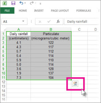
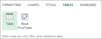
3. Click Tables, move your cursor to the Table button to preview your data, and then click the Table button.

   

4. Click the arrow  in the table header of a column.

5. To filter the data, clear the Select All check box, and then select the data you want to show in your table.

   

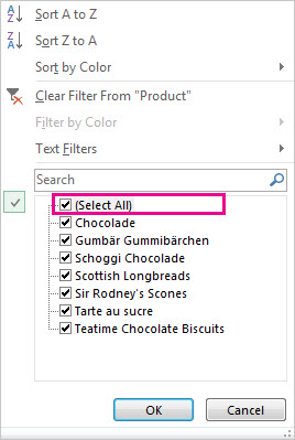
6. To sort the data, click Sort A to Z or Sort Z to A.

   

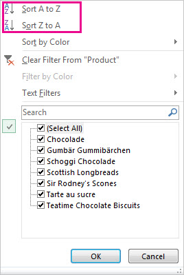
7. Click OK.

Show total for your number using Quick Analysis

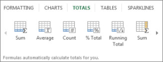
The Quick Analysis tool (available in Excel 2016 and Excel 2013 only) let you total your numbers quickly. Whether it’s a sum, average, or count you want, Excel shows the calculation results right below or next to your numbers.

1. Select the cells that contain numbers you want to add or count.

2. Click the Quick Analysis button  in the bottom-right corner of the selection.

3. Click Totals, move your cursor across the buttons to see the calculation results for your data, and then click the button to apply the totals.

   

Add meaning to  your data using Quick Analysis

Conditional formatting or sparklines can highlight your most important data or show data trends. Use the Quick Analysis tool (available in Excel 2016 and Excel 2013 only) for a Live Preview to try it out.

1. Select the data you want to examine more closely.

2. Click the Quick Analysis button  in the bottom-right corner of the selection.

3. Explore the options on the Formatting and Sparklines tabs to see how they affect your data.

   

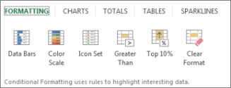   For example, pick a color scale in the Formatting gallery to differentiate high, medium, and low temperatures.

   

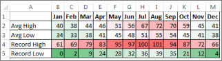
4. When you like what you see, click that option.

Show your data in a chart  using Quick Analysis

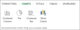
The Quick Analysis tool (available in Excel 2016 and Excel 2013 only) recommends the right chart for your data and gives you a visual presentation in just a few clicks.

1. Select the cells that contain the data you want to show in a chart.

2. Click the Quick Analysis button  in the bottom-right corner of the selection.

3. Click the Charts tab, move across the recommended charts to see which one looks best for your data, and then click the one that you want.

   

Sort your data

To quickly sort your data

1. Select a range of data, such as A1:L5 (multiple rows and columns) or C1:C80 (a single column). The range can include titles that you created to identify columns or rows.

2. Select a single cell in the column on which you want to sort.

3. Click  to perform an ascending sort (A to Z or smallest number to largest).

4. Click  to perform a descending sort (Z to A or largest number to smallest).

5. To sort by specific criteria

6. Select a single cell anywhere in the range that you want to sort.

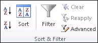
7. On the Data tab, in the Sort & Filter group, choose Sort.

8. The Sort dialog box appears.

9. In the Sort by list, select the first column on which you want to sort.

10. In the Sort On list, select either Values, Cell Color, Font Color, or Cell Icon.

11. In the Order list, select the order that you want to apply to the sort operation — alphabetically or numerically ascending or descending (that is, A to Z or Z to A for text or lower to higher or higher to lower for numbers).

Filter your data

1. Select the data that you want to filter.

2. On the Data tab, in the Sort & Filter group, click Filter.

   

3. Click the arrow  in the column header to display a list in which you can make filter choices.

4. To select by values, in the list, clear the (Select All) check box. This removes the check marks from all the check boxes. Then, select only the values you want to see, and click OK to see the results.

Save your work

1. Click the Save button on the Quick Access Toolbar, or press Ctrl+S.

   

   If you’ve saved your work before, you’re done.

2. If this is the first time you've save this file:

1. Under Save As, pick where to save your workbook, and then browse to a folder.

2. In the File name box, enter a name for your workbook.

3. Click Save.

Print your work

1. Click File, and then click Print, or press  Ctrl+P.

2. Preview the pages by clicking the Next Page and Previous Page arrows.

   

   The preview window displays the pages in black and white or in color, depending on your printer settings.

   If you don’t like how your pages will be printed, you can change page margins or add page breaks.

3. Click Print.

Activate and use an add-in

1. On the File tab, choose Options, and then choose the Add-Ins category.

2. Near the bottom of the Excel Options dialog box, make sure that Excel Add-ins is selected in the Manage box, and then click Go.

3. In the Add-Ins dialog box, select the check boxes the add-ins that you want to use, and then click OK.

   If Excel displays a message that states it can't run this add-in and prompts you to install it, click Yes to install the add-ins.

Find and apply an template

Excel allows you to apply built-in templates, to apply your own custom templates, and to search from a variety of templates on Office.com. Office.com provides a wide selection of popular Excel templates, including budgets.